
The article explains how the encoder in a neural network operates, detailing the steps involved in preparing data and calculating token representations. It starts with the initialization of the dataset and describes the training cycle, including how data is grouped into batches for processing.
Key processes such as embedding, dropout, normalization, and the attention mechanism are discussed, focusing on the roles of various components like SelfAttentionEncoderLayer and LayerNorm. The article also covers linear transformations and the use of relative positional encoding, explaining how input data is transformed through multiple layers before being sent to the decoder. Overall, it provides a thorough understanding of the encoder's functionality and its importance in training models.

Start of encoder operation
After initialization, the following steps take place:
- the dataset is finalized, i.e. the entire training data preparation pipeline is activated;
├── dataset = self._finalize_dataset() module training.py
- the cycle is started with the number of steps specified in the Train steps parameter;
- at each step of the training cycle, groups are extracted from the training dataset grouped into batches;
- the number of groups will be equal to the effective batch size // batch size. For example, if we set the parameter effective batch size = 200 000, and batch size = 6 250, the number of groups will be equal to 200 000 // 6 250 = 32.
- in each of 32 groups will be 6250 tokens, so the total volume of tokens that will be processed for one step of training will be equal to the effective batch size, i.e. 200 000 tokens.
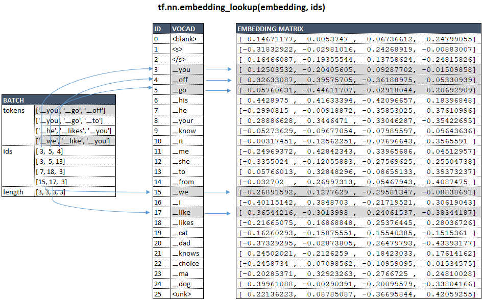
- from the group is extracted from the batches, and for each token in the batches, a vector representation of the token is extracted from the embedding matrix using the function tf.nn.embedding_lookup.
├── call() | class WordEmbedder(TextInputter) module text_inputter.py
Using the example of our model with vocab_size = 26 and num_units = 4, schematically, for source language this can be represented as follows: (Image 1 - embedding matrix)
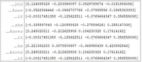
Suppose that our batches consist of 3 training elements.
Source: (Image 2 - source)
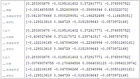
Target: (Image 3 - target)
In ENCODER VECTOR PREPARATION OF TOKENES source LANGUAGE:
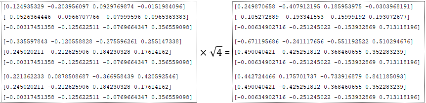
- is multiplied by the square root of the dimension - inputs = inputs * √numunits for example num_units = 4; (Image 4 - num_units = 4)
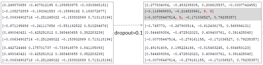
- dropout is applied (dropout parameter from the configuration file), i.e. values are randomly replaced by zero using the function tf.nn.dropout. At the same time, all other values (except those replaced by zero) are adjusted by multiplying by 1/(1 - p), where p is the dropout probability. This is done to bring the values to the same scale, which allows using the same network for training (at probability < 1.0) and inference (at probability = 1.0); (Image 5 - dropout parameter)
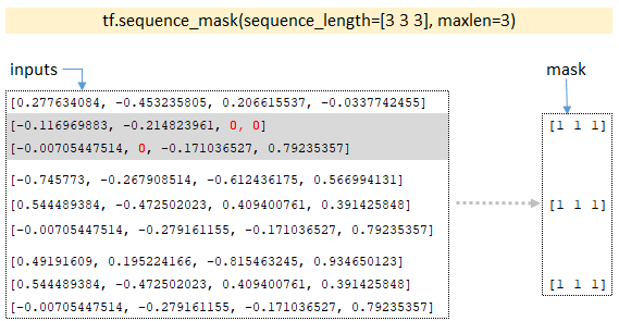
- By the dimensionality of the batches, the tf.sequence_mask function builds the mask tensor; for our example, the dimensionality of the batches will be [3 3 3] and the function returns the mask; (Image 6 - tf.sequence_mask)
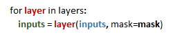
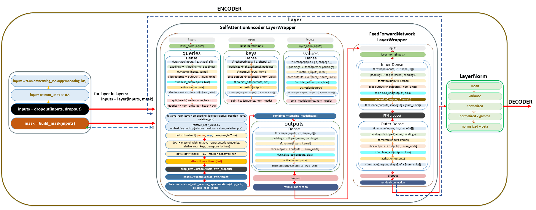
- In the loop, for each layer, equal to the number of Layers parameter, the vector representation of the batched vector (which is stored in the variable inputs) and the mask tensor is passed to the layer, the result returned by the layer is passed to the next layer. For example, if we have 6 layers, the result from the first layer will be the input result for the second layer, etc.
- Each layer represents an object of the SelfAttentionEncoderLayer class, in which the attention mechanism is implemented using the MultiHeadAttention class. The mechanism of transformations occurring in each SelfAttentionEncoderLayer layer is described below.
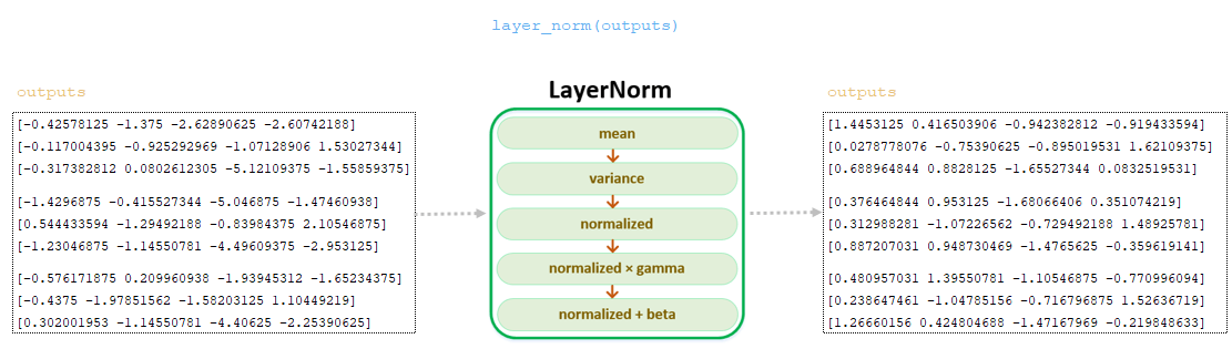
Normalization layer, class LayerNorm()
With parameter Pre norm = True, a normalization layer is applied to the batch after dropout and masking operation, before calculation of attention weights - for each batch runoff with k values we calculate the mean and variance:
mean_i = sum(x_i[j] for j in range(k))/k
var_i = sum((x_i[j] - mean_i) ** 2 for j in range(k))/k
Then the normalized value x_i_normalized, including a small epsilon factor (0.001) for numerical stability, is calculated:
x_i_normalized = (x_i — mean_i) / sqrt(var_i + epsilon)v
And finally, x_i_normalized is linearly transformed using gamma and beta, which are trainable parameters (at initialization gamma = [1, ..., 1], beta = [0, ..., 0]):
output_i = x_i_normalized * gamma + betaoutput_i = x_i_normalized * gamma + beta
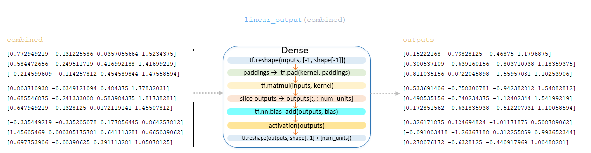
Values of the queries matrix are calculated - normalized values of the inputs matrix obtained at the previous step are passed through the linear transformation of the tf.keras.layers.Dense layer.
Linear transformation, class Dense()
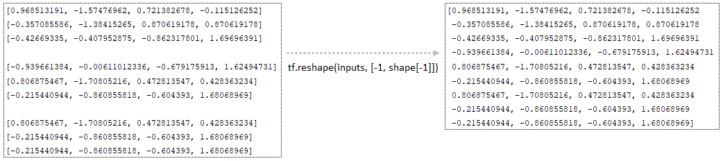
━ 1) the dimensionality of the batches is calculated → shape = [3, 3, 4];
━ 2) changes the dimensionality of tf.reshape (inputs, [-1, shape[-1]]) → tf.reshape(inputs, [-1, 4]); (Image 7 - tf.reshape)
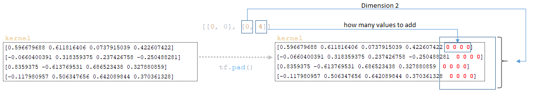
━ 3) with mixed_precision and num_units divisible by 8, the padding size and its formation is calculated
padding_size = 8 - num_units % 8 → padding_size = 8 - 4 % 8 = 4
paddings = [[0, 0], [0, padding_size]] → paddings = [[0, 0], [0, 4]]
the weights of the kernel layer (which were formed during initialization) of the queries matrix are supplemented by padding tf.pad(kernel, paddings); (Image 8 - tf.pad)
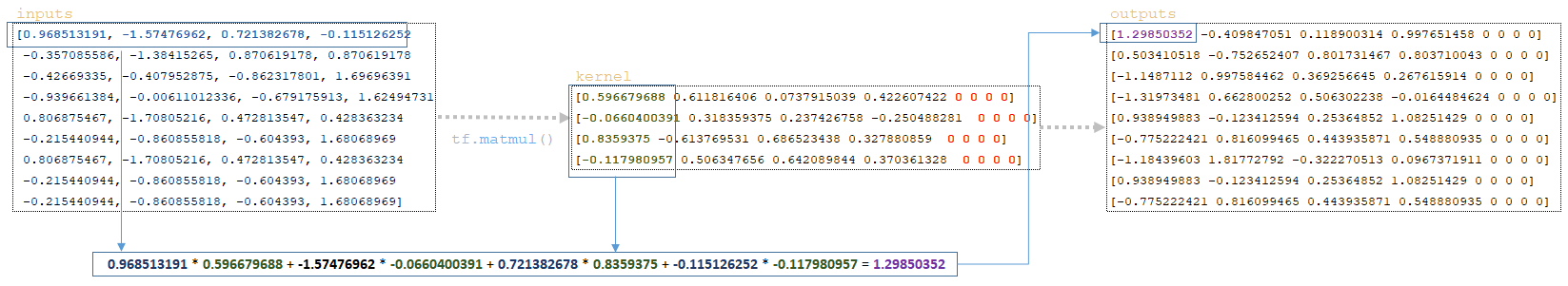
━ 4) the kernel matrices and the batched matrix (inputs) tf.matmul(inputs, kernel) are multiplied; (Image 9 - tf.matmul)
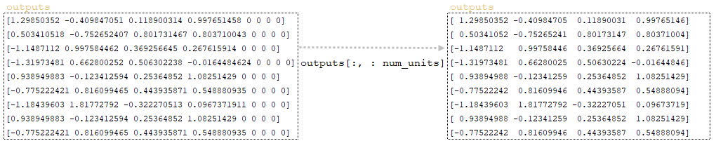
━ 5) a slice of the num_units layer dimension is taken from the resulting matrix and the outputs matrix is formed; (Image 10 - outputs matrix)
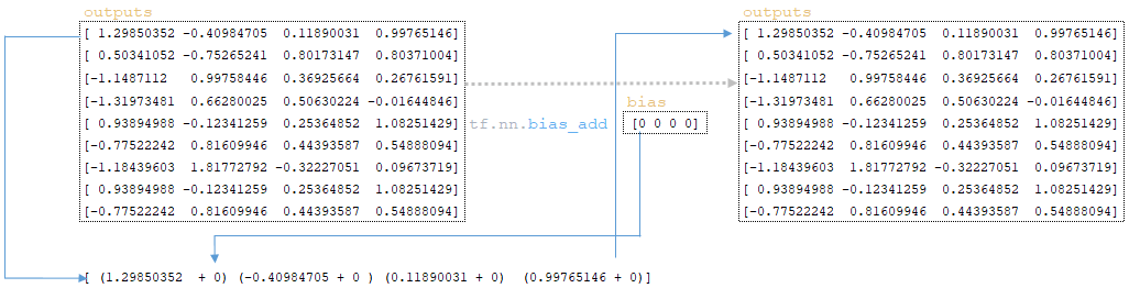
━ 6) the bias vector is added to the outputs matrix obtained at the previous step (initial bias values are initialized with the kernel layer and are initially equal to zero) tf.nn.bias_add(outputs, bias); (Image 11 - tf.nn.bias_add)
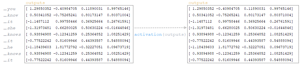
━ 7) after adding bias, the matrix outputs undergoes linear layer activation activation(outputs). Linear layer activation is the application of a function to the matrix. Since the function for the tf.keras.layers.Dense layer is not defined, by default, the activation function is a(x) = x, i.e. the matrix remains unchanged; (Image 12 - activation)
━ 8) after activating the linear layer, the outputs matrix is reshaped tf.reshape(outputs, shape[:-1] + [num_units]) → tf.reshape(outputs, [3, 3, 4]). After this step we get the queries matrix. (Image 13 - queries matrix)
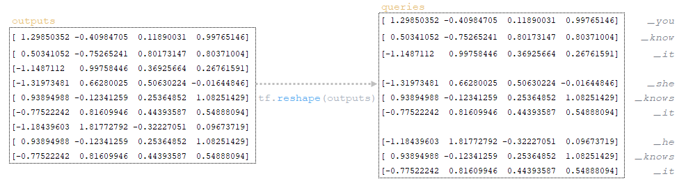
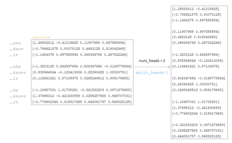
Queries matrix obtained at the previous step is divided by the number of heads (in our architecture the number of heads is 2, the mechanism of division is described in the first part of the article). (Image 14 - queries matrix divided by the number of heads)
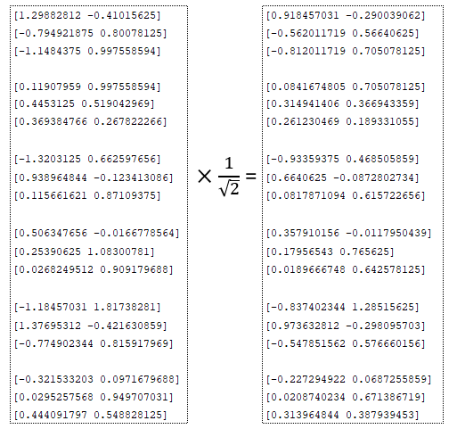
Divided by the number of heads the queries matrix is divided by the square root: (Image 15 - queries matrix divided by square root)
num_units_per_head:
num_units_per_head = num_units // num_heads
num_units_per_head = 4 // 2 = 2
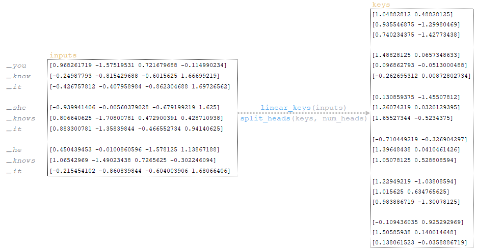
According to steps 1-8 described above (Linear transformation item), the keys matrix is calculated and divided by the number of goals. (Image 16 - keys matrix)
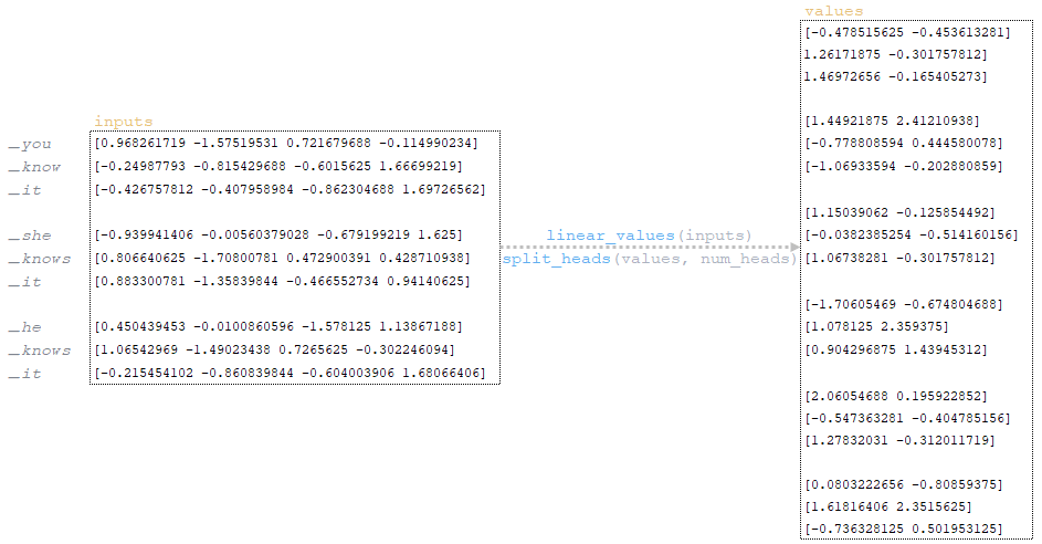
Following steps 1-8 above, the values matrix is calculated and divided by the number of goals. (Image 17 - values matrix)
Relative encoding
Since the example under consideration uses relative positional encoding (maximum_relative_position = 8), the next step is relative encoding:
━ 1) the dimensionality of the keys matrix is calculated:
keys_length = tf.shape(keys)[2]
keys_length = [3 2 3 2 2][2]
keys_length = 3;
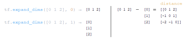
━ 2) an array of integer elements of length keys_length is formed:
arange = tf.range(length)
arange = [0 1 2];
━ 3) two matrices on axis 0 and 1 are formed using the function tf.expand_dims(input, axis) and from the obtained matrices the distance to the diagonal is calculated distance = tf.expand_dims(arange, 0) - tf.expand_dims(arange, 1); (Image 18 - distance matrix)
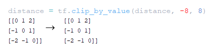
━ 4) distance matrix to the distance diagonal is clipped at the value of maximum_relative_position tf.clip_by_value(distance, -maximum_position, maximum_position); (Image 19 - maximum_relative_position)
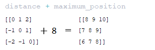
━ 5) the value of maximum_relative_position is added to the distance matrix obtained at the previous step; (Image 20 - distance + maximum_position matrix)
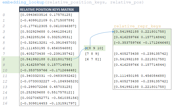
━ 6) the relative_pos matrix obtained at the previous step is used to extract from the relative_position_keys matrix formed at model initialization the corresponding elements by indices using the function tf.nn.embedding_lookup and the relative_repr_keys matrix is formed; (Image 21 - relative_repr_keys matrix)
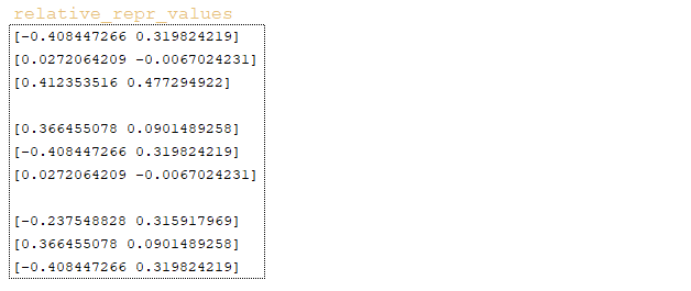
━ 7) the matrix relative_repr_values → embedding_lookup (relative_position_values, relative_pos) is formed in the same way; (Image 22 - relative_repr_values matrix)
Scalar product
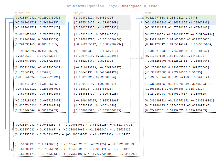
The next step is the scalar product of the matrix queries and keys → dot = tf.matmul(queries, keys, transpose_b=True). (Image 23 - scalar product of queries and keys matrices)
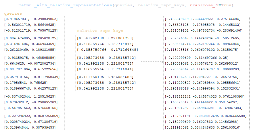
Matrix queries is multiplied with matrix relative_repr_keys → matmul_with_relative_representations (queries, relative_repr_keys, transpose_b=True). (Image 24 - queries matrix multiplied with relative_repr_keys matrix)
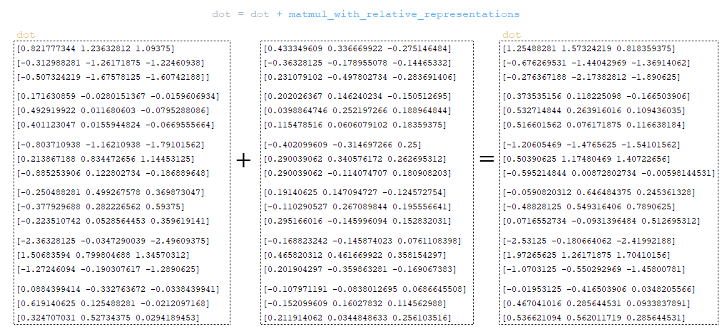
To the dot matrix is added the matrix obtained at matmul_with_relative_representations step. (Image 25 - dot matrix)
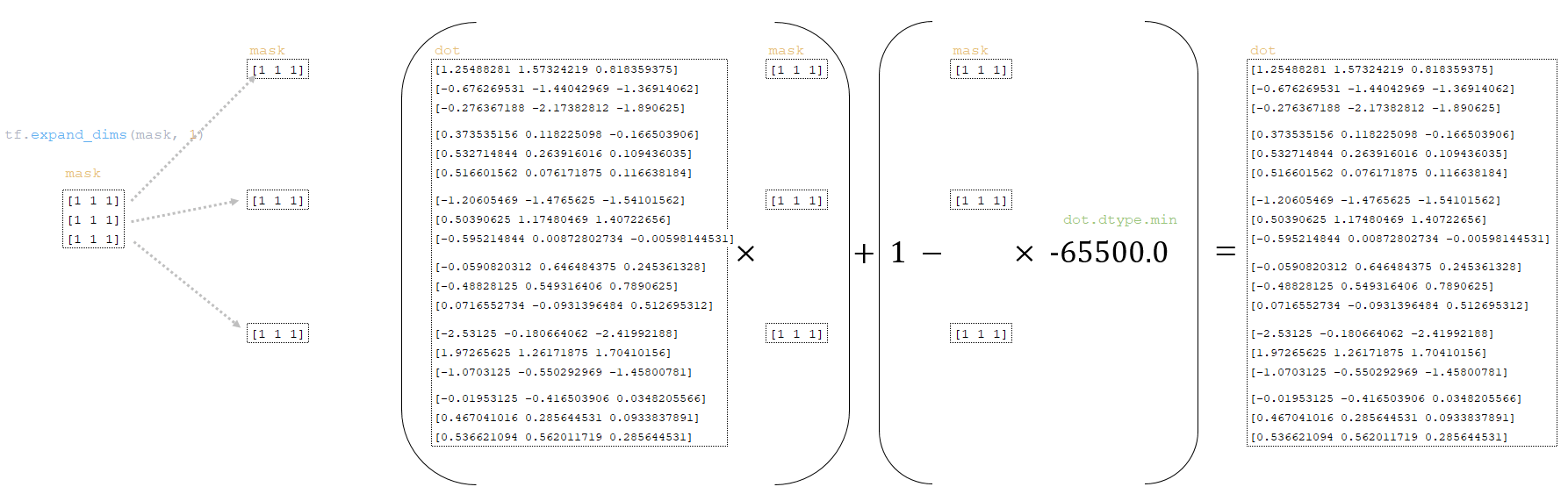
The dot matrix is transformed using the mask matrix obtained from the token batches above:
━ 1) the dimension of the mask matrix is changed mask = tf.expand_dims(mask, 1)
━ 2) the dot the dot matrix is transformed as follows
dot = (dot * mask) + (1.0 - mask) * dot.dtype.min
(Image 26 - dot and mask matrixes)
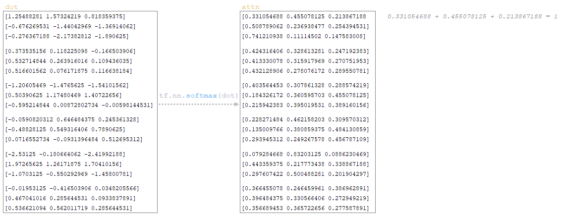
The softmax activation function is applied to the dot matrix and we obtain the matrix attn → attn = tf.nn.softmax(dot). The softmax function is used to transform the vector of values into a probability distribution that sums up to 1. (Image 27 - softmax application)
Dropout is applied to the attn matrix (parameter attention_dropout from the configuration file). (Image 28 - dropout application)

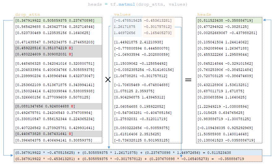
After dropout, the drop_attn matrix is multiplied with the values matrix to form the heads matrix. (Image 29 - matrix heads)
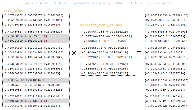
The drop_attn matrix is multiplied with the relative_repr_values matrix. (Image 30 -drop_attn matrix)
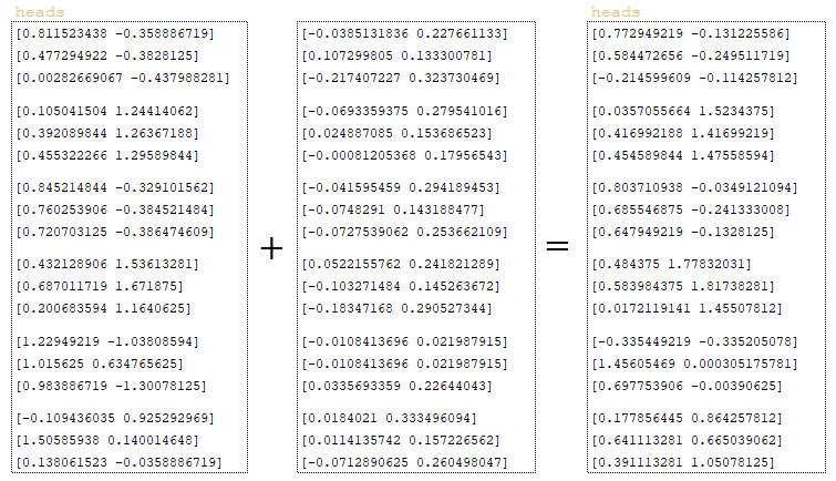
The matrix obtained at matmul_with_relative_representations step is added to the heads matrix. (Image 31 - heads matrix )
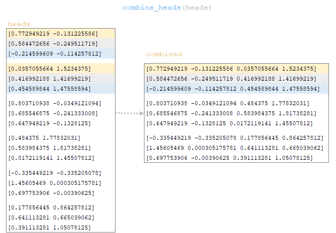
The heads matrix is converted to the dimension of the original batch through the combine_heads function - i.e. perform inverse operations split_heads - get the matrix combined. (Image 32 - matrix combined)
The matrix combined undergoes a linear transformation, after which we get the matrix outputs → outputs = linear_output(combined). The linear transformation is completely identical from the 1st to the 8th step described in the Dense() class. (Image 33 - linear transformation of the combined matrix)
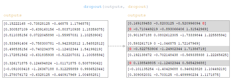
Dropout is applied to the outputs matrix (dropout parameter from the configuration file). (Image 34 - applying dropout to matrix outputs)
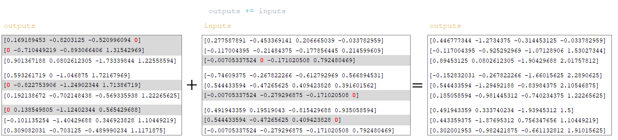
Residual connection mechanism is applied - inputs matrix is added to outputs matrix. Residual connection is a mechanism used to solve the problem of vanishing gradient in deep neural networks and to improve model training and convergence. (Image 35 - outputs + inputs matrix)
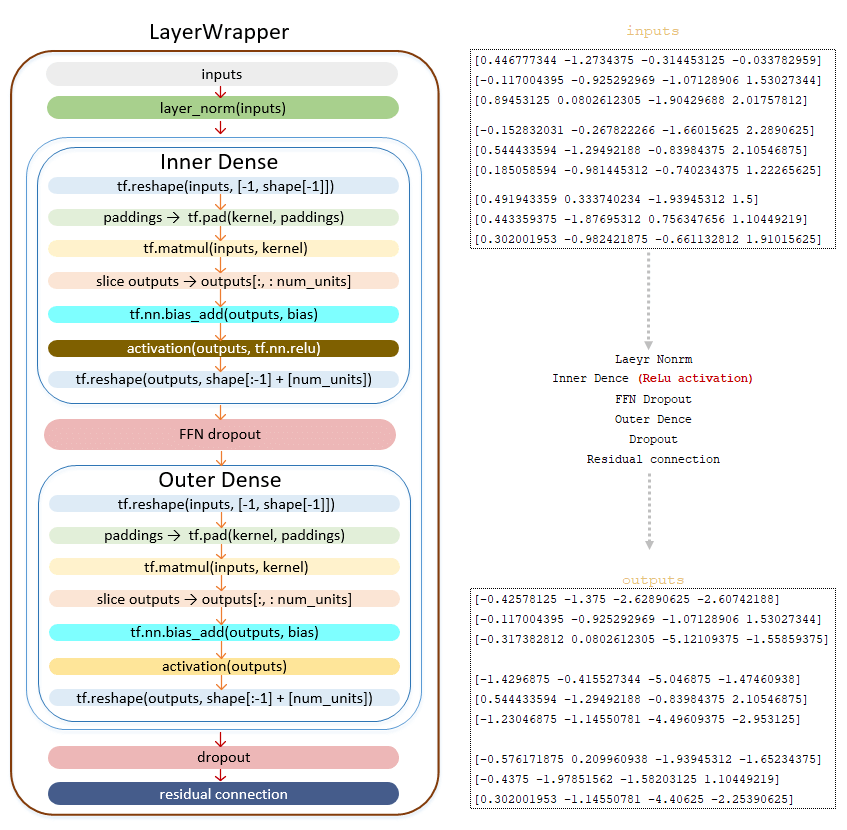
Outputs matrix is passed to the Feed Forward Network:
━ 1) normalization layer LayerNorm() is applied
━ 2) linear transformation Dense() class.
Linear transformation with ReLU activation function tf.nn.relu
━ 3) dropout is applied (parameter ffn_dropout from configuration file)
━ 4) linear transformation of Dense() class
━ 5) dropout is applied (dropout parameter from configuration file)
━ 6) residual connection mechanism is applied
(Image 36- transfer of outputs matrix to Feed Forward Network)
If the value of Layers is greater than one, then after transforming the outputs matrix using Feed Forward Network, the resulting matrix is sent to the input of the next layer until it passes through all layers.
Received matrix outputs from the last layer, passes the normalization layer LayerNorm() - the final operation in the encoder. The matrix obtained at this step is passed to the decoder. (Image 37 - normalization layer LayerNorm())
The above-described mechanism of conversion of the source language token batches in the encoder can be mapped as follows. (Image 38 - mechanism for converting source language tokenization to encoder)
Encoder. Simplified call sequence:
├── def call() | class Model(tf.keras.layers.Layer) module model.py
├── def call() | class SequenceToSequence(model.SequenceGenerator) module sequence_to_sequence.py
├── def call() | class WordEmbedder(TextInputter) module text_inputter.py
├── def call() | class SelfAttentionEncoder(Encoder) module self_attention_encoder.py
├── def build_mask() | class Encoder(tf.keras.layers.Layer) module encoder.py
├── def call() | class LayerWrapper(tf.keras.layers.Layer) module layers /common.py
├── def call() | class SelfAttentionEncoderLayer(tf.keras.layers.Layer) module layers/transformer.py
├── def call() | class MultiHeadAttention(tf.keras.layers.Layer) module layers/transformer.py
├── def call() | class Dense(tf.keras.layers.Dense) module layers /common.py
├── def call() | class LayerWrapper(tf.keras.layers.Layer) module layers /common.py
├── def call() | class FeedForwardNetwork(tf.keras.layers.Layer) module layers/transformer.py
├── def call() | class LayerNorm(tf.keras.layers.LayerNormalization) module layers/common.py
Conclusion
The article provides a comprehensive overview of the encoder's function within a neural network, detailing the various steps involved in processing input data. It outlines how the dataset is finalized and how training occurs in batches, emphasizing the importance of mechanisms such as embedding, dropout, and normalization. Throughout the process, the use of multi-head attention is highlighted, demonstrating how queries, keys, and values are transformed and combined. The article also explains the application of relative positional encoding and the scalar product computations essential for attention mechanisms.
Ultimately, the encoder's output is further processed through normalization and a feed-forward network, with residual connections ensuring effective training. The final output of the encoder is then prepared for the decoder, illustrating the encoder's critical role in transforming input tokens into meaningful representations for subsequent processing.