
The article provides a comprehensive overview of the loss function calculation in machine learning, particularly within the context of sequence models. It begins by detailing how the logits matrix, generated after transformations in the decoder, is processed through the cross_entropy_sequence_loss function. This function plays a crucial role in measuring the discrepancy between predicted outputs and actual labels. The steps involved include converting logits to a suitable format, applying label smoothing to create smoothed labels, and calculating the cross-entropy loss using softmax. Each transformation is meticulously explained, making it clear how each component contributes to the overall loss evaluation.
In addition to the loss calculation, the article examines the alignment mechanism used to enhance model performance. It describes how the loss value is adjusted based on guided alignment, allowing the model to better account for relationships between source and target sequences. The process of calculating and applying gradients is also detailed, illustrating how the optimizer updates model weights to minimize loss.

Loss Function Calculation
The process starts with the logits matrix obtained after transformations in the decoder and the target language batch is passed to the cross_entropy_sequence_loss function. (Image 1 - logits matrix)
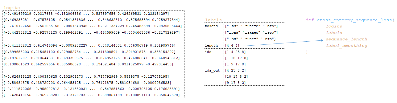
The following transformations take place inside the function:
the cross_entropy matrix is calculated using the softmax_cross_entropy function:
- values of the logits matrix are converted to float32 type using the tf.cast function → logits = tf.cast(logits, tf.float32);
- the value of the variable num_classes is calculated by the dimension of the logits matrix → num_classes = logits.shape[-1] ; since the dimension of the logits matrix is [3, 4, 26], the value of the variable will be equal to 26;
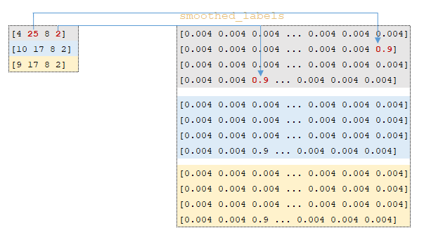
- on_value → 1.0 - label_smoothing (the label_smoothing parameter is taken from the training config); the value of the variable will be equal to 0.9;
- off_value is calculated → label_smoothing / (num_classes - 1 ) ; 1/(26 - 1) = 0.004;
- using function tf.one_hot the smoothed_labels matrix is calculated → tf.one_hot(labels, 26, 0.9, 0.004); this transformation works in the following way - the indices of the output tokens ids_out are extracted from the target language token batches, a matrix with a depth of 26 elements is built and if the index of the matrix element coincides with the index from the ids_out matrix, this index is filled with the value from on_value all other elements are filled with the value from off_value. (Image 2 - smoothed_labels matrix);
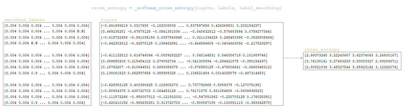
- function tf.nn.softmax_cross_entropy_with_logits calculates the softmax cross entropy between the smoothed_labels and logits matrices. The cross entropy measures the discrepancy between two probability distributions.
The algorithm for this function is as follows:
- the exponent of the logits matrix is calculated - equivalently numpy.exp(logits);
- the matrix elements are summarized line by line - equivalent to numpy.sum(numpy.exp(logits), axis=-1);
- the decimal logarithm of the obtained matrix is taken and transposed by the dimensionality of the logits matrix (in our example 3 x 4 x 1) equivalently numpy.log(numpy.sum(numpy.exp(logits), axis=-1)).reshape(3, 4, 1);
- the matrix obtained at the previous step is subtracted from the logits matrix to form the logsoftmax matrix → logsoftmax = logits - numpy.log(numpy.sum(numpy.exp(logits), axis=-1)).reshape(3, 4, 1)).reshape(3, 4, 1) ;
- cross_entropy matrix is considered - the logsoftmax matrix is multiplied by the negative logits matrix and the product is summarized line by line → cross_entropy = numpy.sum(logsoftmax * -labels, axis=-1). (Image 3 - cross_entropy)
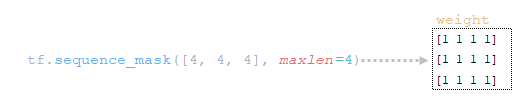
2) using the function tf.sequence_mask, the weight matrix is calculated using the variable sequence_length (this variable contains the values of sentence lengths in tokens grouped in a batch) and the dimensionality of the matrix logits.shape[1] [3, 4, 26]; (Image 4 - weight)

3) using the function tf.math.reduce_sum, the variable loss → loss = tf.reduce_sum( cross_entropy * weight ) = 39.6399841 by the product of the matrices cross_entropy and weight; (Image 5 - product of cross_entropy and weight matrices)
4) using the function tf.math.reduce_sum the variable loss_token_normalizer is calculated using the matrix weight, which will be equal to the number of tokens in the battle → loss_token_normalizer = tf.reduce_sum(weight) = 12;
5) the result returns two variables loss = 39.6399841 and loss_token_normalizer = 12.
Simplified call sequence:
├── def _accumulate_gradients(self, batch) module training.py
├── def compute_gradients(features, labels, optimizer) class Model(tf.keras.layers.Layer) module model.py
├── def compute_training_loss(features, labels) class Model(tf.keras.layers.Layer) module model.py
├── def compute_loss(outputs, labels) class SequenceToSequence(model.SequenceGenerator) module sequence_to_sequence.py
├── def cross_entropy_sequence_loss() module utils/losses.py
Alignment mechanism
When training a model with an alignment, the value in the loss variable , obtained at the previous step, is adjusted using the guided_alignment_cost function. The following transformations take place inside the function:
1) depending on the Guided alignment type parameter set in the configuration file, the conversion function is determined:
- for ce value - tf.keras.losses.CategoricalCrossentropy(reduction=tf.keras.losses.Reduction.SUM) - default value
- for value mse - tf.keras.losses.MeanSquaredError(reduction=tf.keras.losses.Reduction.SUM)
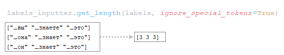
2) the length of sentences in tokens is calculated by the target language token batches; (Image 6 - get_length)
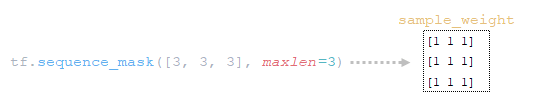
3) using the function tf.sequence_mask, the tf.shape(attention)[1] tensor of weights sample_weight is constructed using the obtained lengths and the dimensionality of the matrix attention tf.shape(attention)[1]; for our example, the length of sentences in tokens will be [3 3 3 3] and the dimensionality of the matrix attention [3 3 3 3]; (Image 7 - sample_weight)
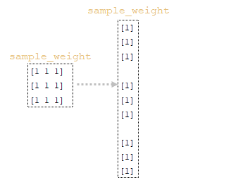
4) with the function tf.expand_dims(input, axis) the matrix sample_weight is resized → sample_weight = tf.expand_dims(sample_weight, -1); (Image 8 - modified sample_weight matrix)
5) using the tf.reduce_sum function, the normalizer → normalizer = tf.reduce_sum([3 3 3 3]) = 9 is calculated from the array of lengths of the batched sentences;
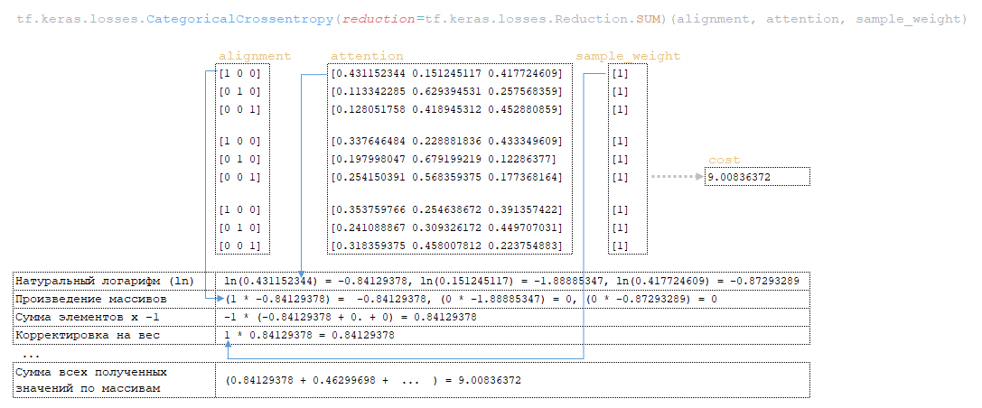
6) using the function tf.keras.losses.CategoricalCrossentropy(alignment, attention), the value of the variable cost is calculated using the matrix alinement (matrix attention (the last element attention[:, :-1] in each vector representation of the token in the matrix attention has been removed beforehand, so that the matrix dimensions coincide, because the dimension of the initial matrix attention is 3 x 4 x 3)) and the matrix sample_weight; (Image 9 - cost variable value calculation)
7) the variable cost is divided by the variable normalizer → cost = cost / normalizer = 9.00836372 / 9 = 1.00092936 ;
8) variable cost is multiplied by the value of variable weight (parameter from the configuration file Guided alignment weight ) → cost = cost * weight = 1.00092936 * 1 = 1.00092936 ;
9) the value from the loss variable obtained in the cross_entropy_sequence_loss function is corrected by the value of the cost variable by adding loss = loss + cost = 39.6399841 + 1.00092936 = 40.6409149.
Simplified call sequence:
├── def _accumulate_gradients(self, batch) module training.py
├── def compute_gradients(features, labels, optimizer) class Model(tf.keras.layers.Layer) module model.py
├── def compute_training_loss(features, labels) class Model(tf.keras.layers.Layer) module model.py
├── def compute_loss(outputs, labels) class SequenceToSequence(model.SequenceGenerator) module sequence_to_sequence.py
├── def guided_alignment_cost() module utils/losses.py
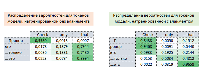
Thus, iteratively, in the process of training the model with an alignment, we adjust the value of the loss function (increasing its value) and thus “force” the optimizer to minimize the loss function taking into account the influence of the alignment. The picture below shows the probability distributions of the attention matrices of target language tokens to source tokens of fully trained models without and with an alignment.
The distributions show that by the probabilities of the attention matrix of the models with an alignment the tokens [▁П, ровер, ьте] can be correctly matched to the token ▁Check, while by the attention matrix of the models without an alignment we cannot. (Image 10 - matrix with and without alignment)
Mechanism for calculating and applying gradients
The process of calculating and applying gradients is as follows:
- the obtained loss value is adjusted by the loss_scale value (initially this value is 32,768) of the LazyAdam optimizer class: scaled_loss = optimizer.get_scaled_loss(loss) → scaled_loss = 40.640914 * 32,768 = 1,331,721.5
- based on the scaled_loss value obtained above and the trainable_weights of the model, gradients are calculated using the gradient function of the tf.GradientTape class. Gradients are derivatives with respect to the model weights. The calculation of gradients is quite complex and is based on the backpropagation algorithm.
The essence of this method is that based on the obtained scaled_loss value and the model weight matrix trainable_weights, the derivatives of the model weights are calculated from left to right, throughout the entire calculation graph. That is, we take the value of the scaled_loss loss function and find the derivatives for the values obtained at the output of the decor, then for the values obtained in the encoder, and so on until the initial values of the model. The goal is to find the value of the derivatives in such a way as to minimize the loss function. Conceptually, the desired neural network training scheme looks something like this: the loss function takes a minimum value → we find the weights corresponding to this value → the error is minimal → the neural network prediction is accurate. Visually, the gradient vector calculation scheme and back propagation mechanism can be displayed as follows.
(Image 11 - calculation of gradient vector)
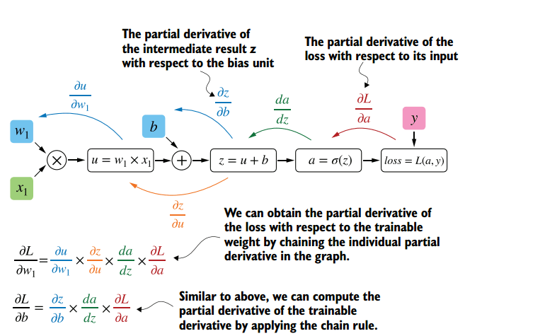
(Image 12 - back propagation mechanism)
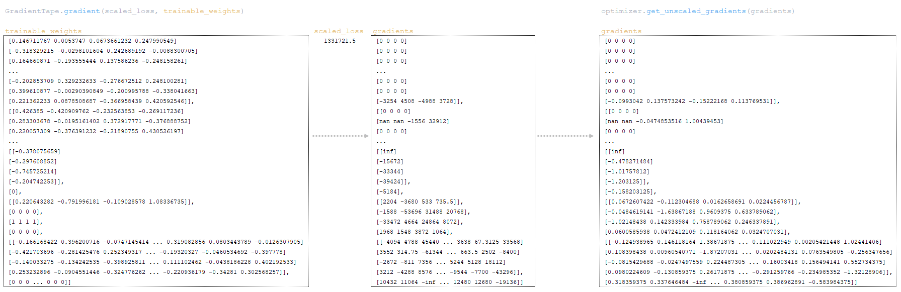
- when training with mixed precision (FP16), the gradients are divided by the loss_scale value using the optimizer function optimizer.get_unscaled_gradients(gradients); below is a slice of the model weights and its gradients (start and end of the matrix); (Image 13 - slice of model weights and its gradients)
- thus, we obtain a gradient matrix, the size of this matrix will be equal to the size of the model weight matrix, i.e. if we have 1 million parameters in the model, then the gradient matrix will contain 1 million values;
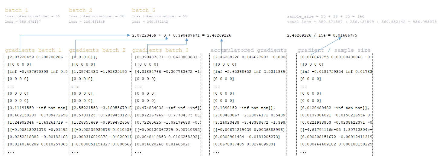
- After calculating the gradient matrix for all groups (batches), the gradients are accumulated. For example, with effective batch size = 200,000 and batch size = 6,250, the number of groups will be 32, i.e. after calculating the gradients, we will have 32 gradient matrices - each batch has its own gradient matrix. Gradients are accumulated by adding the matrices together. In addition to accumulating gradient matrices, they are also accumulated by adding the values obtained in the loss functions loss and loss_token_normalizer (the total number of target tokens in the batch) with the formation of variables:
━ loss = all_reduce_sum(loss)
━ sample_size = all_reduce_sum(loss_token_normalizer)
- after the gradient matrices are summed, loss and loss_token_normalizer the gradient value is divided by the total number of tokens in the sample_size group. For example, below is the mechanism for three batches with a total number of tokens of 146; (Image 14 - three batch mechanism)
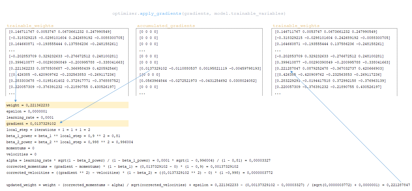
- using the apply_gradients function of the optimizer class, gradients are applied to the model weights, i.e. the model weights are updated. Implementation of the Adam optimizer weight update mechanism. The weight update algorithm using one value from our example as an example:
━ momentums and velocities - are initially initialized to zero. They contain the momentum values for each model weight and will be adjusted and updated with each step;
━ alpha - adaptive value of the learning rate parameter.
(Image 15 - applying gradients to model weights)
When using a different type of optimizer, the mechanism for calculating and applying gradients will be different.
Simplified calling sequence:
├── def call() class Trainer module training.py
├── def _steps() class Trainer module training.py
├── def _accumulate_gradients(batch) class Trainer module training.py
├── def compute_gradients() class Model(tf.keras.layers.Layer) module model.py
├── def _accumulate_loss() class Trainer module training.py
├── def call() class GradientAccumulator module optimizers/utils.py
├── def _apply_gradientss() class Trainer module training.py
After applying gradients, the value of the loss function is divided by the total number of tokens, loss = float(loss) / float(sample_size) → 40.6409149 / 12 = 3.38674291. This is the value that will be displayed in our training log: Step = 1; Loss = 3.386743. And this value will be used to plot the training loss function graph displayed in Tensorboard.
Conclusion
The paper concludes by highlighting the critical processes involved in calculating loss and applying gradients in machine learning models. By understanding how these components interact, particularly the adjustments for alignment and careful computation of gradients, researchers can better optimize their models for improved accuracy and performance.